Trumps Approval List

# Import approval polls data
approval_polllist <- read_csv(here::here('data', 'approval_polllist.csv'))

glimpse(approval_polllist)

## Rows: 14,533
## Columns: 22
## $ president           <chr> "Donald Trump", "Donald Trump", "Donald Trump",...
## $ subgroup            <chr> "All polls", "All polls", "All polls", "All pol...
## $ modeldate           <chr> "8/29/2020", "8/29/2020", "8/29/2020", "8/29/20...
## $ startdate           <chr> "1/20/2017", "1/20/2017", "1/20/2017", "1/21/20...
## $ enddate             <chr> "1/22/2017", "1/22/2017", "1/24/2017", "1/23/20...
## $ pollster            <chr> "Gallup", "Morning Consult", "Ipsos", "Gallup",...
## $ grade               <chr> "B", "B/C", "B-", "B", "B", "C+", "B-", "B+", "...
## $ samplesize          <dbl> 1500, 1992, 1632, 1500, 1500, 1500, 1651, 1190,...
## $ population          <chr> "a", "rv", "a", "a", "a", "lv", "a", "rv", "a",...
## $ weight              <dbl> 0.262, 0.680, 0.153, 0.243, 0.227, 0.200, 0.142...
## $ influence           <dbl> 0, 0, 0, 0, 0, 0, 0, 0, 0, 0, 0, 0, 0, 0, 0, 0,...
## $ approve             <dbl> 45.0, 46.0, 42.1, 45.0, 46.0, 57.0, 42.3, 36.0,...
## $ disapprove          <dbl> 45.0, 37.0, 45.2, 46.0, 45.0, 43.0, 45.8, 44.0,...
## $ adjusted_approve    <dbl> 45.8, 45.3, 43.2, 45.8, 46.8, 51.6, 43.4, 37.7,...
## $ adjusted_disapprove <dbl> 43.6, 37.8, 43.9, 44.6, 43.6, 44.4, 44.5, 42.8,...
## $ multiversions       <chr> NA, NA, NA, NA, NA, NA, NA, NA, NA, NA, NA, NA,...
## $ tracking            <lgl> TRUE, NA, TRUE, TRUE, TRUE, TRUE, TRUE, NA, NA,...
## $ url                 <chr> "http://www.gallup.com/poll/201617/gallup-daily...
## $ poll_id             <dbl> 49253, 49249, 49426, 49262, 49236, 49266, 49425...
## $ question_id         <dbl> 77265, 77261, 77599, 77274, 77248, 77278, 77598...
## $ createddate         <chr> "1/23/2017", "1/23/2017", "3/1/2017", "1/24/201...
## $ timestamp           <chr> "13:38:37 29 Aug 2020", "13:38:37 29 Aug 2020",...

# Use `lubridate` to fix dates, as they are given as characters.

Create a plot

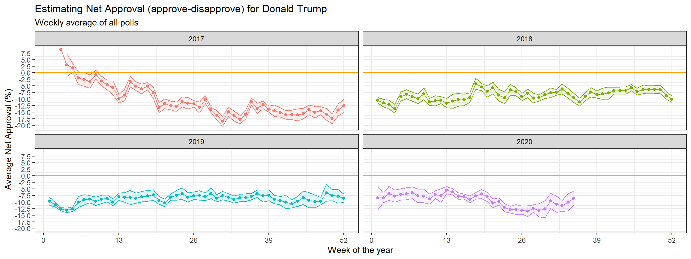
I calculated the average net approval rate (approve- disapprove) for each week since he got into office. I plotted the net approval, along with its 95% confidence interval. As part of the assignment for the MAM.

temp1<-approval_polllist%>%
  filter(enddate!="12/31/2017")%>%
  mutate(enddate=mdy(enddate), #mdy because month/day/year in lubridate
         week_ty=isoweek(enddate),
         year=year(enddate))%>%
  filter(subgroup=="Voters")%>%
  group_by(year,week_ty)%>%
  mutate(netappper=approve-disapprove)%>%
  summarise(week_ty=isoweek(enddate),
            year=as.character(year(enddate)),
            netapp=mean(netappper),
            sdnetapp=sd(netappper))%>%
  mutate(standard_error=sdnetapp/sqrt(n()),
         tcrit=qt(0.975,n()-1)) %>% 
  mutate(lower_95=netapp-tcrit*standard_error, 
         upper_95=netapp+tcrit*standard_error) %>% 
  unique()#note after previous operations, there will be numerous identical rows: the commands make them identical, but mutate/summarise do not delete them, that's why we need unique()
  
  
ggplot(temp1,aes(x=week_ty,y=netapp,color=year))+
  geom_line(show.legend = FALSE)+geom_point(show.legend=FALSE)+
  geom_ribbon(aes(x=week_ty,ymin=lower_95,ymax=upper_95,fill=year),alpha=0.1,show.legend=FALSE)+
  geom_hline(yintercept=0,color="orange")+
  facet_wrap(~year)+
  theme_bw()+
  scale_x_continuous(breaks=seq(0,52,by=13))+
  scale_y_continuous(breaks=seq(-20.0,7.5,by=2.5))+
  labs(title="Estimating Net Approval (approve-disapprove) for Donald Trump",
       subtitle="Weekly average of all polls",
       x="Week of the year",
       y="Average Net Approval (%)")