Mask Acceptance
NYT mask use
Github source for data https://github.com/nytimes/covid-19-data/tree/master/mask-use
Getting the data
#Source for data url <- "https://github.com/nytimes/covid-19-data/raw/master/mask-use/mask-use-by-county.csv"

nyt_mask_survey <- read_csv(here::here("data", "nyt_mask_survey.csv"))

nyt_mask_survey <- nyt_mask_survey %>%
  clean_names() %>%
  mutate(
    mostly_yes= frequently+always,
    mostly_no = never+rarely,
    delta = mostly_yes-mostly_no
  )

glimpse(nyt_mask_survey)
## Rows: 3,142
## Columns: 9
## $ countyfp <chr> "01001", "01003", "01005", "01007", "01009", "01011", "0...
## $ never <dbl> 0.053, 0.083, 0.067, 0.020, 0.053, 0.031, 0.102, 0.152, ...
## $ rarely <dbl> 0.074, 0.059, 0.121, 0.034, 0.114, 0.040, 0.053, 0.108, ...
## $ sometimes <dbl> 0.134, 0.098, 0.120, 0.096, 0.180, 0.144, 0.257, 0.130, ...
## $ frequently <dbl> 0.295, 0.323, 0.201, 0.278, 0.194, 0.286, 0.137, 0.167, ...
## $ always <dbl> 0.444, 0.436, 0.491, 0.572, 0.459, 0.500, 0.451, 0.442, ...
## $ mostly_yes <dbl> 0.739, 0.759, 0.692, 0.850, 0.653, 0.786, 0.588, 0.609, ...
## $ mostly_no <dbl> 0.127, 0.142, 0.188, 0.054, 0.167, 0.071, 0.155, 0.260, ...
## $ delta <dbl> 0.612, 0.617, 0.504, 0.796, 0.486, 0.715, 0.433, 0.349, ...Choropleth map
The FIPS code is a federal code that numbers states and territories of the US. It extends to the county level with an additional four digits, so every county in the US has a unique six-digit identifier, where the first two digits represent the state.
We will be using Kieran Healy’s socviz package which among other things contains county_map and county_data
# America’s choropleths; use county_map that has all polygons
# and county data with demographics/election data from socviz datafile
# The id field is the FIPS code for the county
county_map %>%
  sample_n(5)
## long lat order hole piece group id
## 1 2008713 -340721 81042 FALSE 1 0500000US24025.1 24025
## 2 -1530110 585614 177059 FALSE 1 0500000US53007.1 53007
## 3 1533346 -335318 130381 FALSE 1 0500000US39031.1 39031
## 4 913802 -766189 100759 FALSE 1 0500000US29031.1 29031
## 5 -314978 59324 105506 FALSE 1 0500000US30011.1 30011county_data %>%
sample_n(5)## id name state census_region pop_dens pop_dens4
## 1 28045 Hancock County MS South [ 50, 100) [ 45, 118)
## 2 47019 Carter County TN South [ 100, 500) [118,71672]
## 3 17049 Effingham County IL Midwest [ 50, 100) [ 45, 118)
## 4 51079 Greene County VA South [ 100, 500) [118,71672]
## 5 32033 White Pine County NV West [ 0, 10) [ 0, 17)
## pop_dens6 pct_black pop female white black travel_time land_area
## 1 [ 82, 215) [ 5.0,10.0) 45949 50.5 88.2 8.1 29.1 474
## 2 [ 82, 215) [ 0.0, 2.0) 56886 51.1 96.8 1.5 22.8 341
## 3 [ 45, 82) [ 0.0, 2.0) 34320 50.2 98.1 0.4 17.8 479
## 4 [ 82, 215) [ 5.0,10.0) 19031 50.6 89.1 6.8 29.3 156
## 5 [ 0, 9) [ 2.0, 5.0) 10034 42.7 87.2 4.5 21.4 8876
## hh_income su_gun4 su_gun6 fips votes_dem_2016 votes_gop_2016
## 1 44522 [11,54] [10,12) 28045 3320 13720
## 2 31842 [ 8,11) [ 8,10) 47019 3453 16897
## 3 52108 [ 0, 5) [ 0, 4) 17049 3071 13613
## 4 59358 [ 8,11) [ 8,10) 51079 2923 5943
## 5 48586 [11,54] [12,54] 32033 707 2723
## total_votes_2016 per_dem_2016 per_gop_2016 diff_2016 per_dem_2012
## 1 17517 0.190 0.783 10400 0.228
## 2 20993 0.164 0.805 13444 0.232
## 3 17428 0.176 0.781 10542 0.232
## 4 9503 0.308 0.625 3020 0.365
## 5 3773 0.187 0.722 2016 0.265
## per_gop_2012 diff_2012 winner partywinner16 winner12 partywinner12 flipped
## 1 0.755 8980 Trump Republican Romney Republican No
## 2 0.752 10710 Trump Republican Romney Republican No
## 3 0.753 8636 Trump Republican Romney Republican No
## 4 0.618 2274 Trump Republican Romney Republican No
## 5 0.702 1618 Trump Republican Romney Republican Noglimpse(county_data)## Rows: 3,195
## Columns: 32
## $ id <chr> "0", "01000", "01001", "01003", "01005", "01007", ...
## $ name <chr> NA, "1", "Autauga County", "Baldwin County", "Barb...
## $ state <fct> NA, AL, AL, AL, AL, AL, AL, AL, AL, AL, AL, AL, AL...
## $ census_region <fct> NA, South, South, South, South, South, South, Sout...
## $ pop_dens <fct> "[ 50, 100)", "[ 50, 100)", "[ 50, 100)",...
## $ pop_dens4 <fct> "[ 45, 118)", "[ 45, 118)", "[ 45, 118)", "[118...
## $ pop_dens6 <fct> "[ 82, 215)", "[ 82, 215)", "[ 82, 215)", "[ 82...
## $ pct_black <fct> "[10.0,15.0)", "[25.0,50.0)", "[15.0,25.0)", "[ 5....
## $ pop <int> 318857056, 4849377, 55395, 200111, 26887, 22506, 5...
## $ female <dbl> 50.8, 51.5, 51.5, 51.2, 46.5, 46.0, 50.6, 45.2, 53...
## $ white <dbl> 77.7, 69.8, 78.1, 87.3, 50.2, 76.3, 96.0, 27.2, 54...
## $ black <dbl> 13.2, 26.6, 18.4, 9.5, 47.6, 22.1, 1.8, 69.9, 43.6...
## $ travel_time <dbl> 25.5, 24.2, 26.2, 25.9, 24.6, 27.6, 33.9, 26.9, 24...
## $ land_area <dbl> 3531905, 50645, 594, 1590, 885, 623, 645, 623, 777...
## $ hh_income <int> 53046, 43253, 53682, 50221, 32911, 36447, 44145, 3...
## $ su_gun4 <fct> NA, NA, "[11,54]", "[11,54]", "[ 5, 8)", "[11,54]"...
## $ su_gun6 <fct> NA, NA, "[10,12)", "[10,12)", "[ 7, 8)", "[10,12)"...
## $ fips <dbl> 0, 1000, 1001, 1003, 1005, 1007, 1009, 1011, 1013,...
## $ votes_dem_2016 <int> NA, NA, 5908, 18409, 4848, 1874, 2150, 3530, 3716,...
## $ votes_gop_2016 <int> NA, NA, 18110, 72780, 5431, 6733, 22808, 1139, 489...
## $ total_votes_2016 <int> NA, NA, 24661, 94090, 10390, 8748, 25384, 4701, 86...
## $ per_dem_2016 <dbl> NA, NA, 0.2396, 0.1957, 0.4666, 0.2142, 0.0847, 0....
## $ per_gop_2016 <dbl> NA, NA, 0.734, 0.774, 0.523, 0.770, 0.899, 0.242, ...
## $ diff_2016 <int> NA, NA, 12202, 54371, 583, 4859, 20658, 2391, 1175...
## $ per_dem_2012 <dbl> NA, NA, 0.266, 0.216, 0.513, 0.262, 0.123, 0.763, ...
## $ per_gop_2012 <dbl> NA, NA, 0.726, 0.774, 0.483, 0.731, 0.865, 0.235, ...
## $ diff_2012 <int> NA, NA, 11012, 47443, 334, 3931, 17780, 2808, 714,...
## $ winner <chr> NA, NA, "Trump", "Trump", "Trump", "Trump", "Trump...
## $ partywinner16 <chr> NA, NA, "Republican", "Republican", "Republican", ...
## $ winner12 <chr> NA, NA, "Romney", "Romney", "Obama", "Romney", "Ro...
## $ partywinner12 <chr> NA, NA, "Republican", "Republican", "Democrat", "R...
## $ flipped <chr> NA, NA, "No", "No", "Yes", "No", "No", "No", "No",...# we have data on 3195 FIPS....
glimpse(county_map)## Rows: 191,382
## Columns: 7
## $ long <dbl> 1225889, 1235324, 1244873, 1244129, 1272010, 1276797, 1273832...
## $ lat <dbl> -1275020, -1274008, -1272331, -1267515, -1262889, -1295514, -...
## $ order <int> 1, 2, 3, 4, 5, 6, 7, 8, 9, 10, 11, 12, 13, 14, 15, 16, 17, 18...
## $ hole <lgl> FALSE, FALSE, FALSE, FALSE, FALSE, FALSE, FALSE, FALSE, FALSE...
## $ piece <fct> 1, 1, 1, 1, 1, 1, 1, 1, 1, 1, 1, 1, 1, 1, 1, 1, 1, 1, 1, 1, 1...
## $ group <fct> 0500000US01001.1, 0500000US01001.1, 0500000US01001.1, 0500000...
## $ id <chr> "01001", "01001", "01001", "01001", "01001", "01001", "01001"...# ... but to create a map, we translate these 3195 counties to 191,382 polygons!Joing the files
We have three files
nyt_mask_survey, our NYT survey data,county_mapthat has all polygons that define a countycounty_datawith demographics/election data.
county_full <- left_join(county_map, county_data, by = "id")

county_masks_full <- left_join(county_full, nyt_mask_survey,
                                by = c("id"="countyfp"))
Building our choropleth plot
p <- ggplot(data = county_masks_full,
            mapping = aes(x = long, y = lat,
                          fill = delta,
                          group = group))

p1 <- p +
  geom_polygon(color = "gray90", size = 0.05) +
  coord_equal()


p2 <- p1 +
  scale_fill_gradient(low = '#ffffcc', high= '#006837')

p3 <- p1 +
  scale_fill_gradient2()

# get different colours from https://colorbrewer2.org/
# the one shown here is https://colorbrewer2.org/#type=diverging&scheme=BrBG&n=6
p4 <- p1 +
  scale_fill_gradientn(colours = c('#8c510a','#d8b365','#f6e8c3','#c7eae5','#5ab4ac','#01665e'))

p1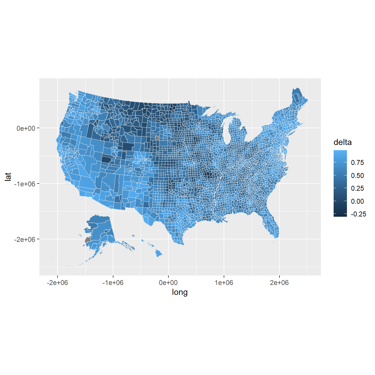
p2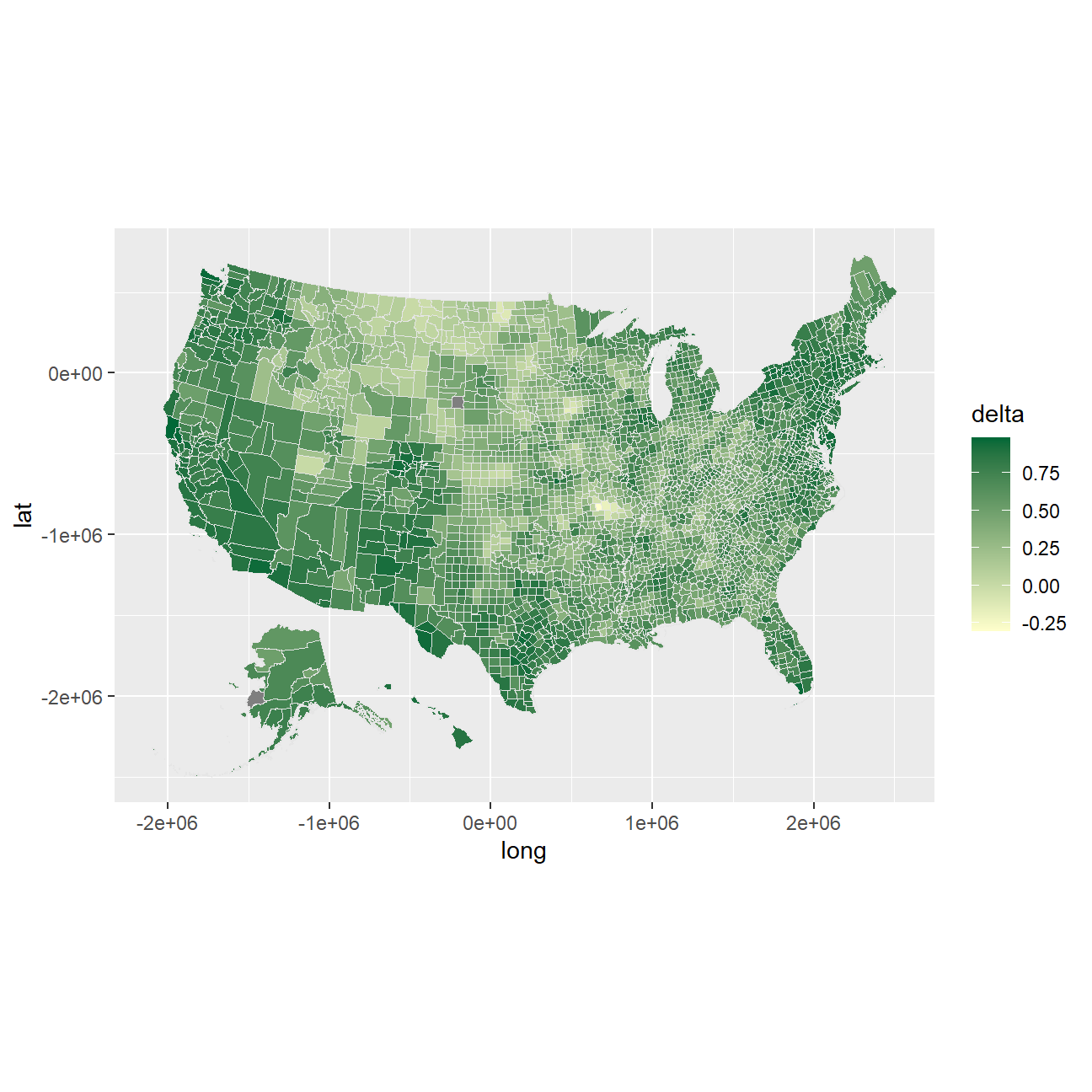
p3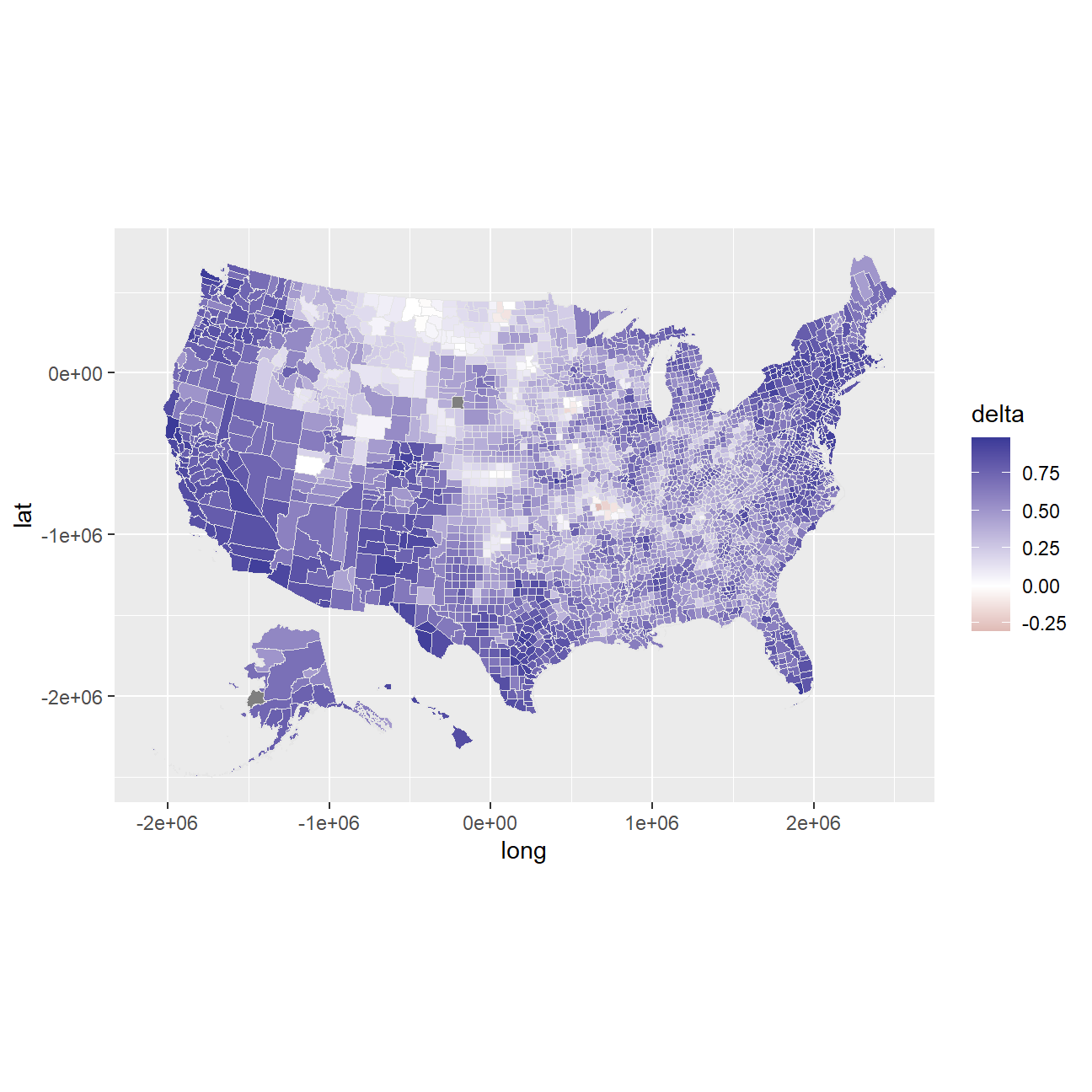
p4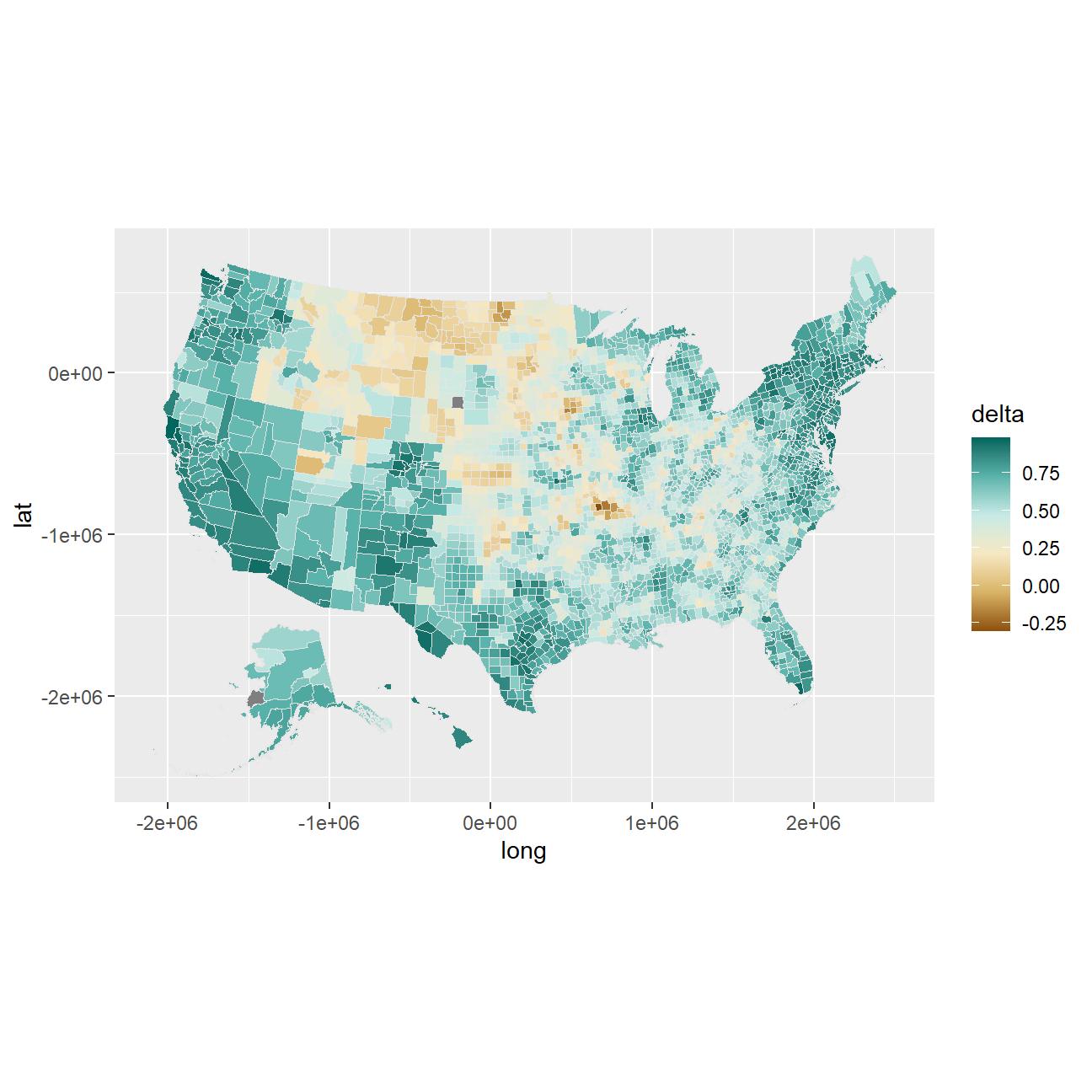
p4 + labs(fill = "Mask acceptance, (Mostly Yes - Mostly No)",
          caption = "“Estimates from The New York Times, based on roughly 250,000 interviews \nconducted by Dynata from July 2 to July 14, 2020”") +
  guides(fill = guide_legend(nrow = 1)) +
  theme_map() +
  theme(legend.position = "bottom")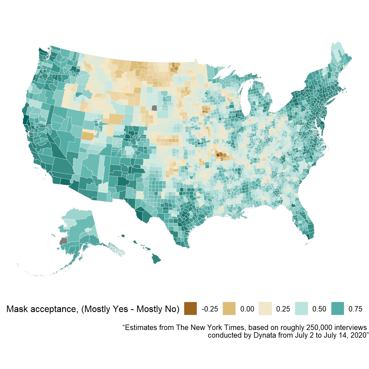
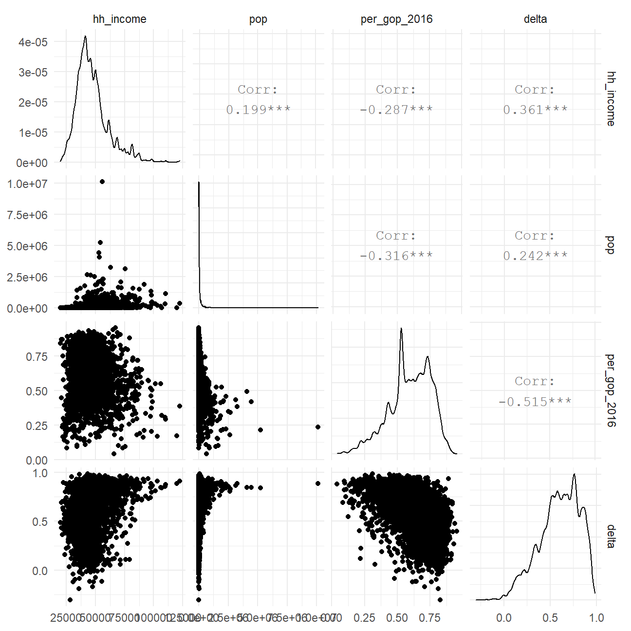
Checking for relationships
Does mask use acceptance have any relation with some demographics? Let us explor the relationship between country household income, population, and % who voted republican in 2016
county_masks_full %>%
  select(hh_income, pop, per_gop_2016, delta) %>%
  GGally::ggpairs()+
  theme_minimal()