TFL Bikes

Recall the TfL data on how many bikes were hired every single day. We can get the latest data by running the following

url <- "https://data.london.gov.uk/download/number-bicycle-hires/ac29363e-e0cb-47cc-a97a-e216d900a6b0/tfl-daily-cycle-hires.xlsx"

# Download TFL data to temporary file
httr::GET(url, write_disk(bike.temp <- tempfile(fileext = ".xlsx")))

## Response [https://airdrive-secure.s3-eu-west-1.amazonaws.com/london/dataset/number-bicycle-hires/2020-09-18T09%3A06%3A54/tfl-daily-cycle-hires.xlsx?X-Amz-Algorithm=AWS4-HMAC-SHA256&X-Amz-Credential=AKIAJJDIMAIVZJDICKHA%2F20200919%2Feu-west-1%2Fs3%2Faws4_request&X-Amz-Date=20200919T174441Z&X-Amz-Expires=300&X-Amz-Signature=c3ae7b68af5142ecf2f8fd43860a9127f0d8ad19b01d44af31f7b152797fe364&X-Amz-SignedHeaders=host]
##   Date: 2020-09-19 17:44
##   Status: 200
##   Content-Type: application/vnd.openxmlformats-officedocument.spreadsheetml.sheet
##   Size: 165 kB
## <ON DISK>  C:\Users\samgo\AppData\Local\Temp\RtmpsvzuLM\file393c476641f.xlsx

# Use read_excel to read it as dataframe
bike0 <- read_excel(bike.temp,
                   sheet = "Data",
                   range = cell_cols("A:B"))

# change dates to get year, month, and week
bike <- bike0 %>% 
  clean_names() %>% 
  rename (bikes_hired = number_of_bicycle_hires) %>% 
  mutate (year = year(day),
          month = lubridate::month(day, label = TRUE),
          week = isoweek(day))

ggplot(filter(bike,year==2015:2020), aes(x=bikes_hired))+ 
  geom_density()+
  facet_grid(cols= vars(month), rows=vars(year), scales="free_y")+
  theme_minimal()+
  labs(y="", x="Bike Rentals")+
  theme(axis.text.y=element_blank())+
  scale_x_continuous(labels=c("20K","40K","60K"),breaks=seq(20000,60000,by=20000))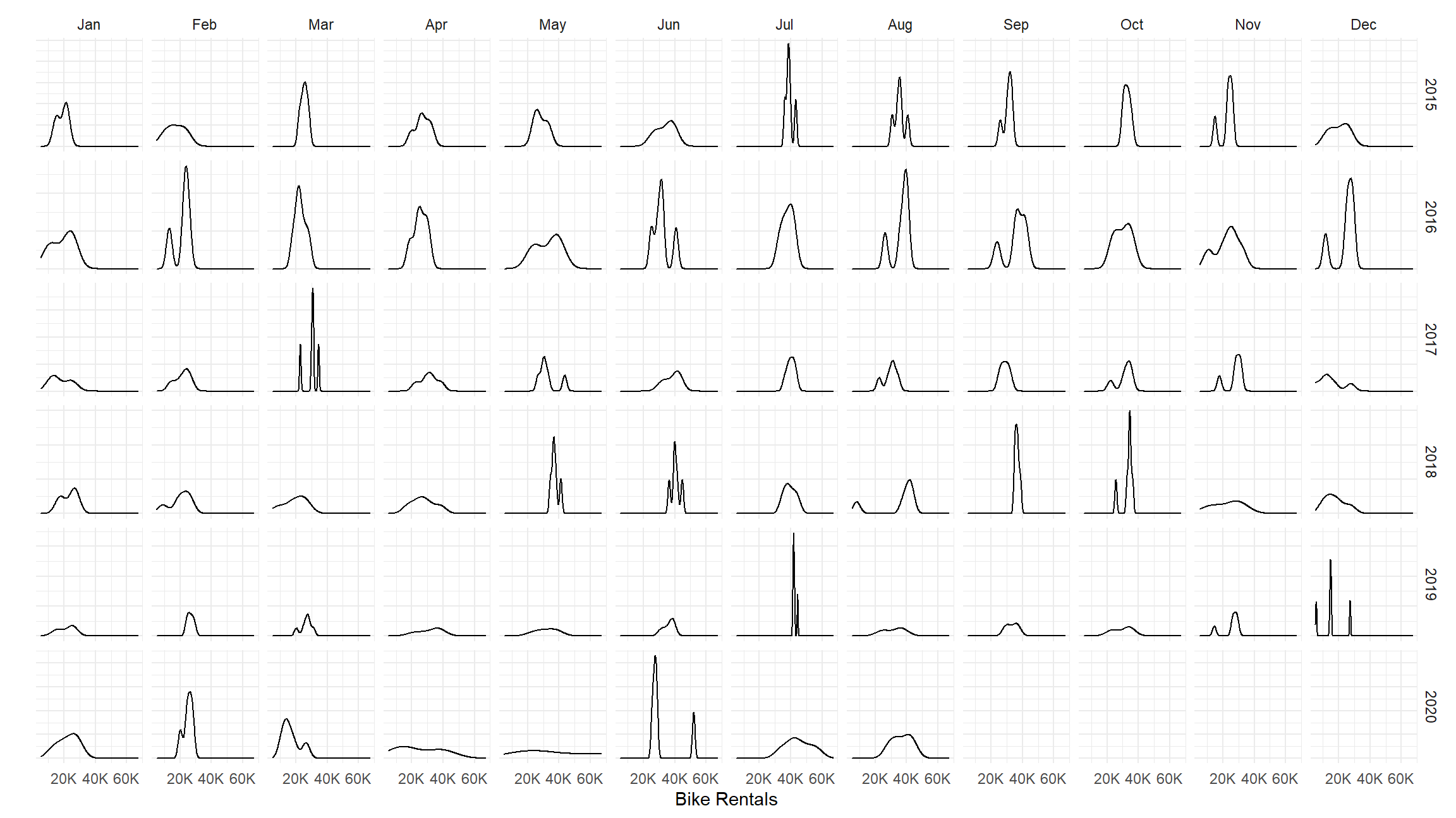

#calculate the bike rental per month
bike_1<-bike%>%
  filter(year>=2015)%>%
  group_by(year,month)%>%
  summarise(year=year,month=month,bikes_month=mean(bikes_hired))%>%
  unique()

# calculate the average bank rental
bike_1m<-bike_1%>%
  ungroup(year)%>%
  filter(year!=2020)%>%
  summarise(month=month,bikes_year=mean(bikes_month))%>%
  unique()

bike_1f<-left_join(x = bike_1, y = bike_1m, by = "month", all.x = TRUE)

  
# make the plot  
ggplot(bike_1f, aes(month, bikes_month)) +  facet_wrap(~year) +
  geom_ribbon(aes(ymin = bikes_month, ymax = pmin(bikes_year, bikes_month), fill = "red"), alpha=0.4, group=1) +
  geom_ribbon(aes(ymin = bikes_year, ymax = pmin(bikes_year, bikes_month), fill = "green"),alpha=0.4, group=1) +
  geom_line(group=1) +
  geom_line(aes(month, bikes_year),colour="blue", size=1, group=1) +
  labs(title="Mothly changes in TfL bike rentals",
       subtitle="Change from monthly average shown in blue \n and calculated between 2015-2019",
       caption = "Source: TfL, London Data Store",
       x="", 
       y="Bike rentals")+
  scale_y_continuous(labels=c("20000","25000","30000","35000","40000"),breaks = seq(20000,40000,by=5000))+
  theme_minimal()+
  theme(title= element_text(size = 15, colour = 'black'))+
  guides(fill=F)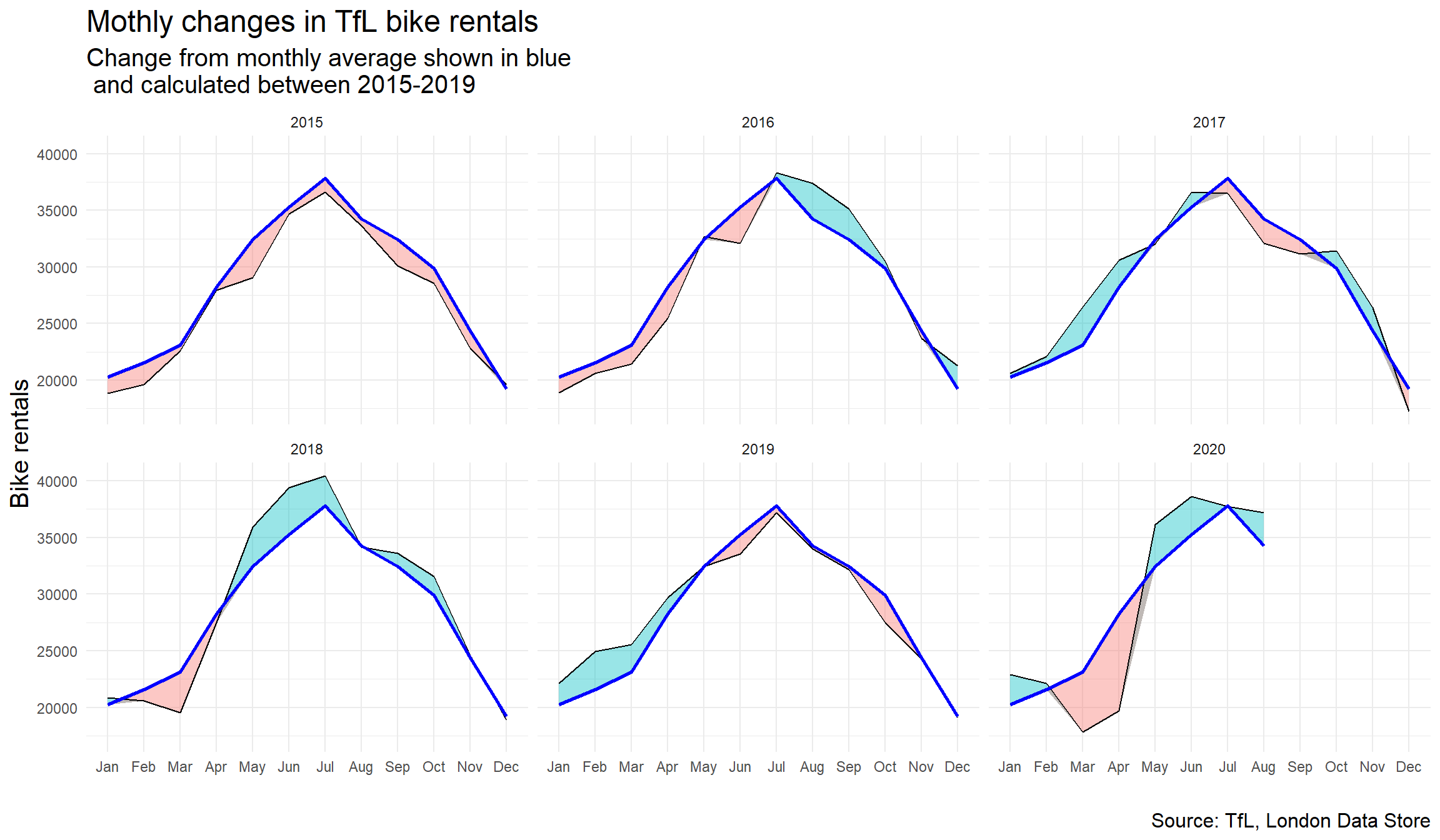

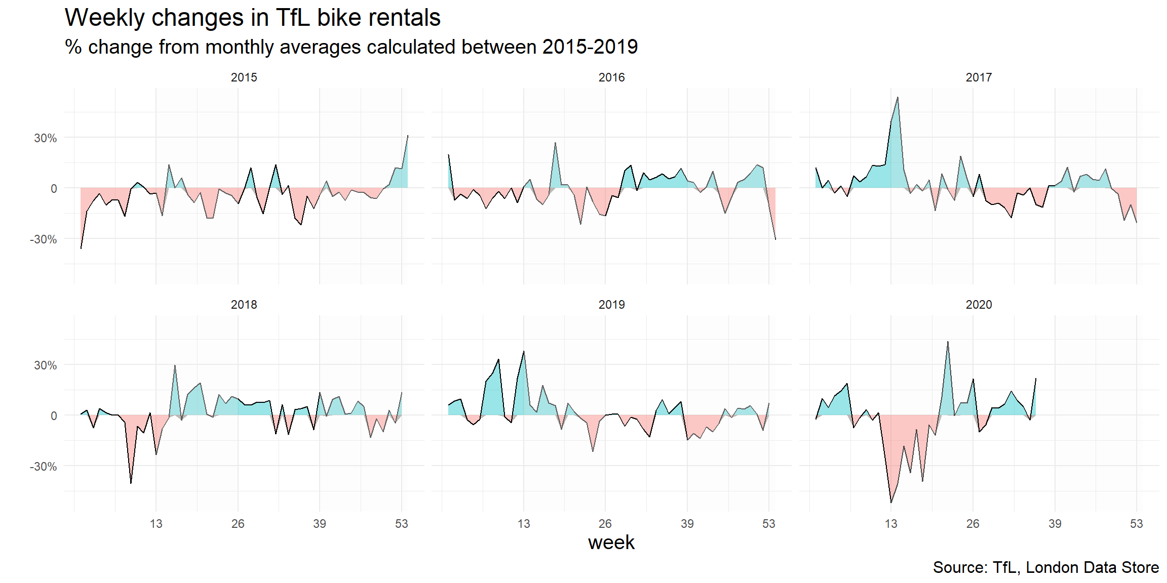
The second one looks at percentage changes from the expected level of weekly rentals. The two grey shaded rectangles correspond to the second (weeks 14-26) and fourth (weeks 40-52) quarters.

#calculate the bikes hired per week in 2015-2019
bike_2<-bike%>%
  filter(year>=2015)%>%
  group_by(year,week)%>%
  summarise(year=year,week=week,bikes_week=mean(bikes_hired))%>%
  unique() %>% 
  ungroup

#calculate the bikes hired 
bike_2<-bike_2 %>% 
  group_by(week) %>% 
  mutate(exp_bikes_week=mean(bikes_week),
         bikes_week_percent=100*(bikes_week-exp_bikes_week)/exp_bikes_week)
  


ggplot(bike_2, aes(week, bikes_week_percent)) +  facet_wrap(~year) +
  geom_ribbon(aes(ymin = bikes_week_percent, ymax = pmin(bikes_week_percent, 0), fill= "red"), alpha=0.4, group=1) +
  geom_ribbon(aes(ymin = 0, ymax = pmin(bikes_week_percent, 0), fill = "green"),alpha=0.4, group=1) +
  #geom_rug(data=.%>% filter(bikes_week_percent>0),
  #         mapping=aes(x=week,y=bikes_week_percent),color="#a1d99b",sides="b")+
  #geom_rug(data=.%>% filter(bikes_week_percent<0),
   #        mapping=aes(x=week,y=bikes_week_percent),color="#a50f15",sides="b")+  
  geom_line(group=1) +
  geom_line(aes(week, bikes_week_percent),size=0.1,group=1) +
  geom_rect(aes(xmin=13, xmax=26, ymin=-Inf, ymax=Inf),fill='light grey',alpha = .01)+
  geom_rect(aes(xmin=39, xmax=53, ymin=-Inf, ymax=Inf),fill='light grey',alpha = .01)+
  theme_minimal()+
  labs(title="Weekly changes in TfL bike rentals",
       subtitle="% change from monthly averages calculated between 2015-2019",
       caption = "Source: TfL, London Data Store",
       x="week", 
       y="")+
  scale_y_continuous(labels=c("-60%","-30%","0","30%","60%"))+
  scale_x_continuous(labels=c("13","26","39","53"),breaks = seq(13,53,by=13))+
  theme(title= element_text(size = 15, colour = 'black'))+
  guides(fill=F)